Transcriptomics

Transcriptomics lecture

---

Transcriptomics Practical

Introduction

An application of next-generation sequencing is RNA sequencing (Mortazavi et al., 2008; Wang et al., 2009). In particular, we will discuss transcriptome (messenger RNA) sequencing. Transcriptome sequencing is a very useful addition to genome sequencing projects as it helps to identify genes and thus aids in genome annotation. In this sense, it is similar to earlier transcriptome sequencing using capillary methods (EST sequencing), but provides much higher coverage of the transcriptome.

Reads from RNA sequencing can be treated in much the same way as those from DNA sequencing. In eukaryotes, however, the effects of splicing (i.e. reads mapping to the edges of exons on both sides of an intron or alternative splicing) needs to be taken into account.

Due to the vast number of reads produced by next generation sequencing technology, the transcriptome is also sequenced very deeply. Each gene is sequenced in proportion to its abundance and the large number of reads means that even low abundance genes are sequenced to some extent. This means that expression levels of genes can be compared. One can visualise the "pile up" of reads in a particular region by looking at coverage plots. The higher the signals in the plot, the more expressed a transcript is. It is important to note that the sequences originate from transcriptome samples (mRNA) and therefore only contain information about the exons and untranslated regions (UTRs).

Imagine the following transcript being present in the sample:

Reads belonging to the transcript are produced by the sequencing process. When the reads come out as raw data, there is no information about where they belong in the reference genome. Furthermore, all reads from several different transcripts come out together. An alignment algorithm localises them in the reference genome based on similarity matches.

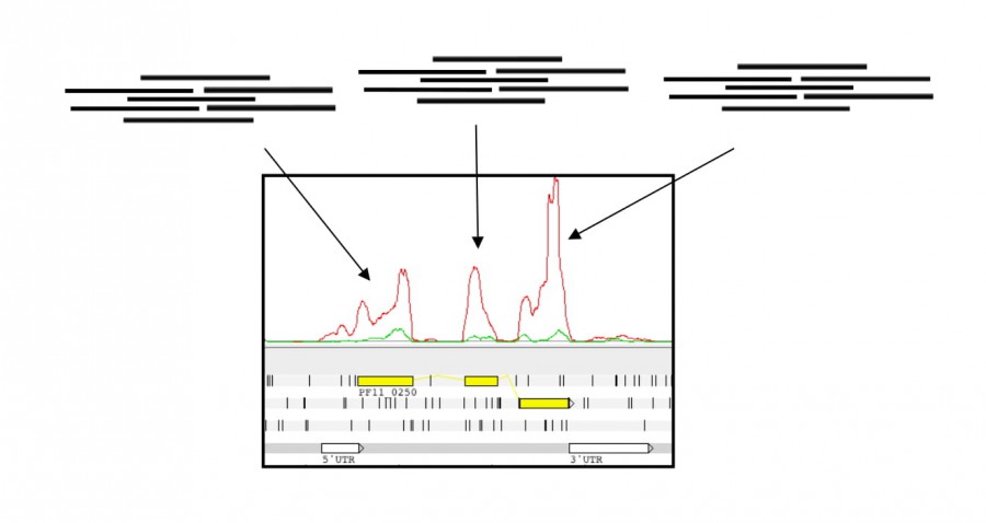
In the plot, the coverage line represents the number of reads that align to the genome at each base position. This allows us to identify coding regions, here, the 3 exons (in yellow) that comprise the transcript above.

In this module we will use a similar approach used to map DNA sequencing data to map RNA sequencing data from Mycobacterium tuberculosis.

Understanding an organism's genome goes beyond cataloging the genes that are present in that genome. Insight into the biological stages in which each gene is expressed (potentially used) helps us to identify how organisms develop and respond to particular external stimuli. The first layer of such complex patterns involves the understanding of how the genome is being used: the transcriptome. This is also the most accessible type of information because, like the genome, the transcriptome is made of nucleic acids and can be sequenced relatively easily. Arguably the proteome is of greater relevance to understand cellular biology, but its chemical heterogeneity makes it much more difficult to assay.

Over the past two decades, microarray technology has been applied extensively for addressing the question of which genes are expressed and when, enabling the performance of differential expression analysis. Despite its success, this technology is limited in that it requires prior knowledge of the gene sequences for an organism and has a limited dynamic range in detecting the level of expression, e.g. how many copies of a transcript are made. RNA sequencing technology using, for instance, Illumina HiSeq machines can sequence all the genes that are transcribed, and the results have a more linear relationship to the real number of transcripts generated.

The aim of differential expression analysis is to determine which genes are more or less expressed in different situations. We could ask, for instance, whether a bacterium uses its genome differentially when exposed to stress, such as heat or challenged by a drug. Alternatively, we could ask which genes make human livers different from kidneys.

In this exercises, we will try to gain some understanding of differences between M. tuberculosis lineages. The genome of M. tuberculosis was published in 1998 (Cole et al., 1998). It has 4.4 Mb and a relatively high GC content (~65%), comprising 4,111 genes. Although the variability of the M. tuberculosis genome has been considered limited, it has demonstrated a higher diversity than was previously thought. Currently, M. tuberculosis is classified in 9 different lineages with different geographical distributions. Strains from different lineages have shown differences in virulence, capacity, and in the acquisition of drug resistance (Parwati et al., 2010). These differences might be caused by variable expression of certain genes.

Therefore, the aim of this session is to become familiar with the steps carried out in transcriptomics studies, from mapping RNA-seq reads to the performance of differential expression analysis.

Exercise 1: Mapping RNA-seq with BWA

First, we will map RNA sequence reads from an M. tuberculosis lineage 1 strain to the reference genome (which has been created from the H37Rv strain).

You can find the M. tuberculosis H37Rv reference genome (called H37Rv.fa) as well as the two files of RNA-seq reads from the lineage 1 strain (Mtb_L1_1.fastq and Mtb_L1_2.fastq) in the transcriptomics directory.

Running BWA

To work with the command line of Linux, you will need to open a terminal, activate this practical's conda environment, and go to the transcriptomics directory:

conda activate rnaseq && cd ~/data/transcriptomics

And list the files there:

ls

You will find the 4 fastq files, 2 of them from the lineage 1 sample, and the reference genome fasta file; these are the input data for this practical.

For the mapping step, first an index of the reference genome must be constructed with bwa index. On the command line, you should type:

bwa index H37Rv.fa

This will generate 5 files which are needed for BWA. We will then align the RNA-seq reads to the reference genome with bwa mem. We will therefore use the reference genome (in fasta format) and the two fastq files that contain the RNA-seq reads, saving the output to a SAM file. To start you should type:

bwa mem H37Rv.fa Mtb_L1_1.fastq.gz Mtb_L1_2.fastq.gz > ./Mapping_Mtb/Mtb_L1.sam

The output will be located in the Mapping_Mtb folder, which is in the transcriptomics directory.

Exercise 2: Converting BWA SAM output to BAM and indexing

SAM to BAM using samtools

The details of where each M. tuberculosis read has been mapped are now stored in a file in the directory Mapping_Mtb. We are going to view the mapped reads in Artemis using the Artemis BAM view. However, the mapping result is not currently in BAM format. To make a BAM file from the BWA output we need to run a short series of programs.

To convert the SAM file created by BWA to BAM format we are going to use samtools. First, we go to the directory where the output file from the BWA command is stored and transform the SAM file to BAM:

cd ~/data/transcriptomics/Mapping_Mtb
samtools view -b Mtb_L1.sam > Mtb_L1.bam

Once we have the BAM file, we need to sort it and index it with the following commands:

samtools sort -o Mtb_L1.sorted.bam Mtb_L1.bam
samtools index Mtb_L1.sorted.bam

To see the list of options and parameters for the commands, type:

samtools view
samtools sort

Now we are going to save our sorted file as Mtb_L1.bam and Mtb_L1.bam.bai for the index one.

mv Mtb_L1.sorted.bam Mtb_L1.bam
mv Mtb_L1.sorted.bam.bai Mtb_L1.bam.bai

The resulting bam and index files will then be in the folder Mapping_Mtb. The alignment output could now be visualised in Artemis, Tablet or a visualisation tool of your choice.

Exercise 3: Visualisation of the BAM files

Now we will examine the reads mapping in Artemis using the BAM view feature.

Viewing the mapped reads in Artemis

Open Artemis (type art in the terminal) and select: 'File', 'Open Project Manager', select '+' to add a new project you can call "Mtb" and load H37Rv.fa, which contains the reference genome. We also need to add the genome features so that we can see the gene models. For doing so, we will load the Mtb.gtf file (is in the transcriptomics directory) as the annotation track. Select 'annotation' and then press 'new property'.

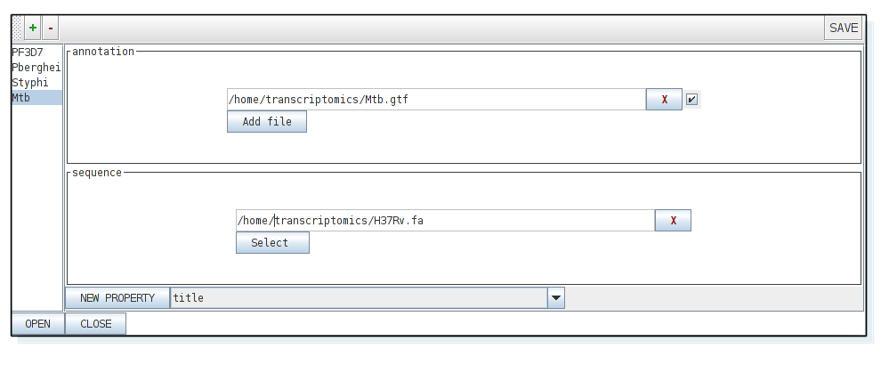
Now select 'open' and the artemis window should appear. From the Artemis 'File' menu, select 'Read BAM/VCF', and then select the bam file you just generated from the L1 Mtb sample (i.e. Mtb_L1.bam).

You should see the BAM window appear (shown in the screen shot below). We want to change the view in order to better see how the reads map to the genome.

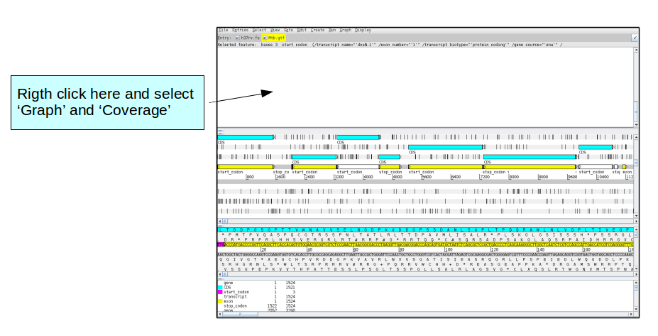
Interpreting the mapping

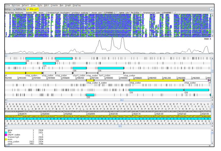
This exercise is similar to the one performed before in the Visualisation module. Scroll along the genome and examine the read coverage (the part of the genome mapped goes from position 2,420,631 to 2,920,631; we have removed reads mapping to other regions from the raw data in order to speed up analysis time). To view the relevant part select 'Goto', 'Navigator' and write in 'Goto Base' 2420631). Notice how different genes have different depths of coverage.

Including more lineages

One interesting feature of the Artemis viewer is the possibility to see more than one BAM file at the same time, which enables to compare coverage from different samples. Hence, next we want to include more lineages, in this case we will add another sample belonging to the lineage 4 of Mtb.

Once we have the bam files, we can add it to the viewer.

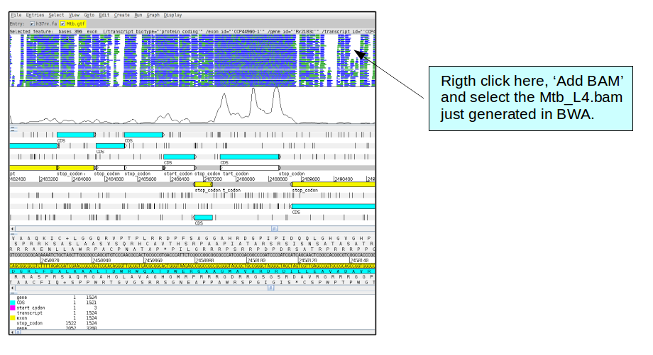
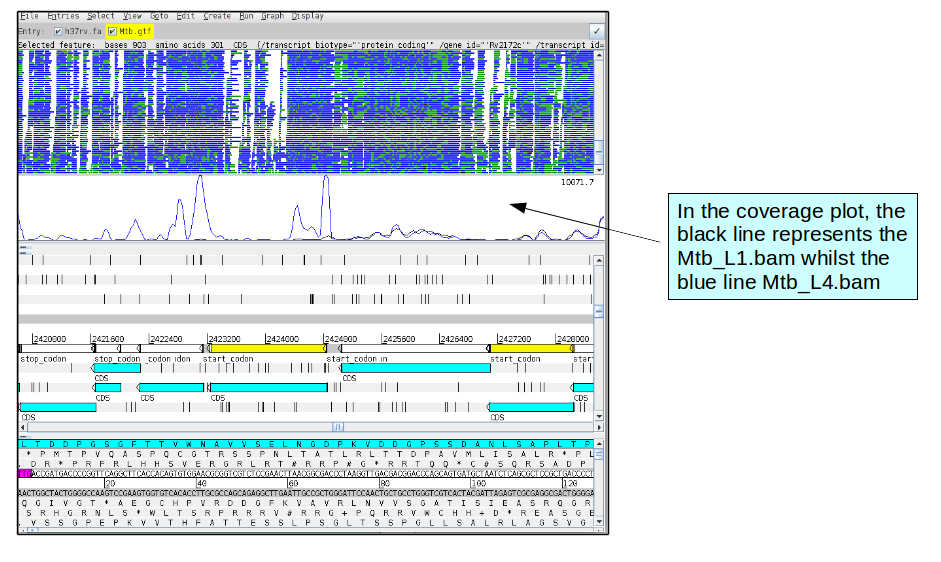
In the BAM view of the reads, it might be difficult to distinguish the differences between the BAM files. However, in the coverage plot, one can see the differences in coverage.

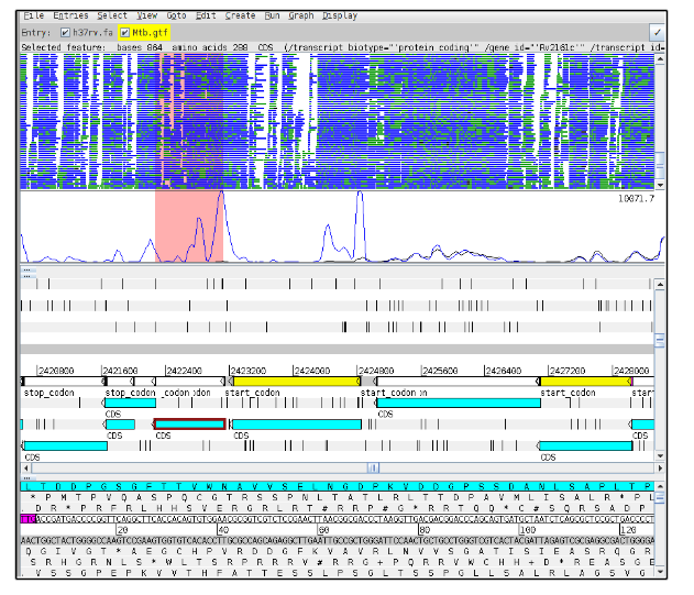
One reason to perform RNA-seq under different conditions or in different samples (in this case different lineages of Mtb), is to see genes that are differentially expressed. For example, one gene may be more highly expressed in one lineage that in the other.

Now go to gene Rv2161c (position 2422271).

Exercse 4: Differential expression

There are tools that calculate the differential expression, like the R packages DESeq or EdgeR. They take the reads mapped to each gene, normalize the resulting quantities of mapped reads (coverage), and then estimate if any genes are differentially expressed. In general, the results are more credible and significant if biological replicates are included.

Counting reads with HTSeq-count

In order to perform a differential expression analysis, the first step is to count the reads mapped to each of the genes so that we can make comparisons between the different samples.

HTSeq-count is part of the HTSeq package which will quantify the number of reads mapping to gene models in different RNA-seq experiments given a file with aligned sequencing reads (the bam file obtained through BWA) and a list of genomic features (the Mtb.gtf file with the gene annotation).

We will run HTSeq-count with the RNA-seq data from the L1 and L4 strains we were using in the previous exercises. to do this, we will go to the directory where we have the data and use the following command:

cd ~/data/transcriptomics
python -m HTSeq.scripts.count -f bam -r pos -s reverse -t gene ./Mapping_Mtb/Mtb_L1.bam Mtb.gtf > ./Mapping_Mtb/Mtb_L1_htseq_count.txt
python -m HTSeq.scripts.count -f bam -r pos -s reverse -t gene ./Mapping_Mtb/Mtb_L4.bam Mtb.gtf > ./Mapping_Mtb/Mtb_L4_htseq_count.txt

The parameters we have used in the HTSeq-count command are:

• -f: format of the input data
• -r: how is sorted the data
• -s: whether the data is from a strand-specific assay. The reverse option is used for pair-end reads from HiSeq in order to mantain the strain-specificity (the reads have to map to the gene in the corresponding strand to be counted)
• -t: feature type, in this case exon

If you have any doubt about the parameters of the program, you can visit https://htseq.readthedocs.io/en/release_0.11.1/count.html

We can now take a look at the results from the HTSeq-count typing the following in the command line:

cd ~/data/transcriptomics/Mapping_Mtb
less Mtb_L1_htseq_count.txt

You should see two columns with the list of genes and the counts for each gene.

To exit this view you just need to type 'q'.

Finding differentially expressed genes with DESeq2

Now we are going to perform a differential expression analysis in order to look for genes with variable expression between lineages. To do it we will use 6 sequenced samples, 3 from lineage 1 and 3 from lineage 4. Two of them will be the two analysed in the previous steps. We are going to use an R package for the anaylsis of the differential gene expression called DESeq2.

A differential expression analysis is used to compare gene expression levels, given by the number of reads per gene (obtained by HTSeq-count) between samples (for example, between 2 lineages of Mtb). In order to accurately ascertain which genes are differentially expressed, and the amount of expression, it is necessary to use replicated data. As with all biological experiments, doing it once may simply not be enough. There is no simple way to decide how many replicates to do, it is usually a compromise of statistical power and cost. By determining how much variability there is in the sample preparation and sequencing reactions we can better assess whether genes are really expressed and more accurately determine any differences. The key to this is performing biological rather than technical replicates. This means, for instance in tuberculosis, growing up three cultures of bacteria, treating them all identically, extracting RNA from each and sequencing the three samples separately. Technical replicates, whereby the same sample is sequenced three times do not account for the variability that really exists in biological systems or the experimental error between cultures of bacteria and RNA extractions. More replicates will help to improve statistical power for genes that are already detected at high levels, while deeper sequencing will improve power to detect differential expression for genes which are expressed at low levels. In this exercise we will consider the 3 L1 and the 3 L4 samples as biological replicates.

To start, we firstly need a table with the counts. In the Mapping_Mtb directory (where we should be) we can find a folder called HTSeqCounts with 6 files called:

cd ~/data/transcriptomics/Mapping_Mtb/HTSeqCounts
ls

Now, to start, we need to open R in the terminal, just typing:

R

And then load the packages we are going to need for the analysis:

library(DESeq2)
library(gplots)

These 6 files are the results of the HTSeq-count of the two samples previously analysed plus 4 more Mtb samples we will use to perform the analysis.

To prepare the data we are going to use the following commands.

First we are going to set the directory where we have the files:

directory <- "~/data/transcriptomics/Mapping_Mtb/HTSeqCounts/" 

And now we can select the files and save them in the variable ‘sampleFiles’ by selecting all the files that contain "Mtb" that are present in our directory:

sampleFiles <- grep("Mtb", list.files(directory), value = TRUE)

As we are comparing lineage 1 to lineage 4 samples, we are going to set up lineage as "condition".

sampleCondition <- c("l4","l1","l1","l4","l1","l4")

Now we construct the table with the sample information and convert it in a DESeq object:

sampleTable <- data.frame(sampleName = sampleFiles,
                          fileName = sampleFiles,
                          condition = sampleCondition)
dds <- DESeqDataSetFromHTSeqCount(sampleTable = sampleTable,
                                      directory = directory,
                                      design = ~ condition)

Before doing the analysis, we are going to filter the dataset keeping only the genes with at least 10 counts, so that we make sure that every gene considered for the analysis was transcribed.

to do this, type the following:

keep <- rowSums(counts(dds)) >= 10
dds <- dds[keep,]

And we are going to set up the condition for the analysis in two levels which are 'lineage 1' and 'lineage 4':

dds$condition <- factor(dds$condition, levels = c("l1","l4"))

We can then run the differential expression anaylisis by calling the function DESeq(), which will normalise the data and compare between the two groups established (l1 and l4). We can store the results in a variable called 'res':

dds <- DESeq(dds)
res <- results(dds)

Let's take a look at the results. Type:

res

And you should get a table like this:

The first column represents the name of each gene analysed, which are represented in rows.

Let's take a look at the summary of the results we just obtained:

summary(res)

When asking whether a gene is differentially expressed we use statistical tests to assign a p-value. If a gene has a p-value of 0.05, we know that there is only a 5% chance that our observations are due to random chance and it is not really differentially expressed. However, if we are asking this question for every gene in the genome, then we would expect to see, due to multiple comparison, p-values less than 0.05 for many genes even though they are not really differentially expressed. Therefore, we must correct the p-values so that we are not tricked into accepting a large number of erroneous results. Adjusted p-values are p-values which have been corrected for what is known as multiple hypothesis testing.

The summary shows us the number of genes with an adjusted p-value < 0.1 that are under- or overexpressed in one of the groups (log2FoldChange above or below 0, here represented as LFC). The adjusted p-value in the DESeq analysis is equivalent to the FDR or 'False Discovery Rate'. This value represents the proportion of discoveries that we can expect to be false.

Some of the p-values in our results might be NA values, which can be due to extreme outliers. To continue with the analysis we are going to remove these missing values.

res <- res[!is.na(res$padj),]

Let's now order the results by p value so that we see the top genes with the highest statistial significance. Take a look at the results again.

resOrdered <- res[order(res$pvalue),]
resOrdered

To visualise the diffences in expression we are going to plot a heatmap using the 17 genes that are above the cut off. To achieve this, we will first get the normalised counts in a variable called "counts_heatmap". We will copy the names of the first 17 genes from our "resOrdered" table in a vector, and then extract the normalised counts from "counts_heatmap" for the 17 genes we want to plot.

counts_heatmap <- counts(dds, normalized = TRUE)
idx <- rownames(resOrdered)[1:17]
counts_heatmap <- counts_heatmap[rownames(counts_heatmap)%in%idx,]

If we type:

counts_heatmap

We can see the table with the normalised counts for each sample and each of the genes of our interest.

To plot the heatmap copy the following commands:

colnames(counts_heatmap) <- c("L4_1","L1_2","L1_3","L4_4","L1_5","L4_6")
heatmap.2(as.matrix(counts_heatmap), scale="row", col=greenred(75), Rowv=NA,
dendrogram = "col", trace="none", density.info = "none")

You should get a plot like this:

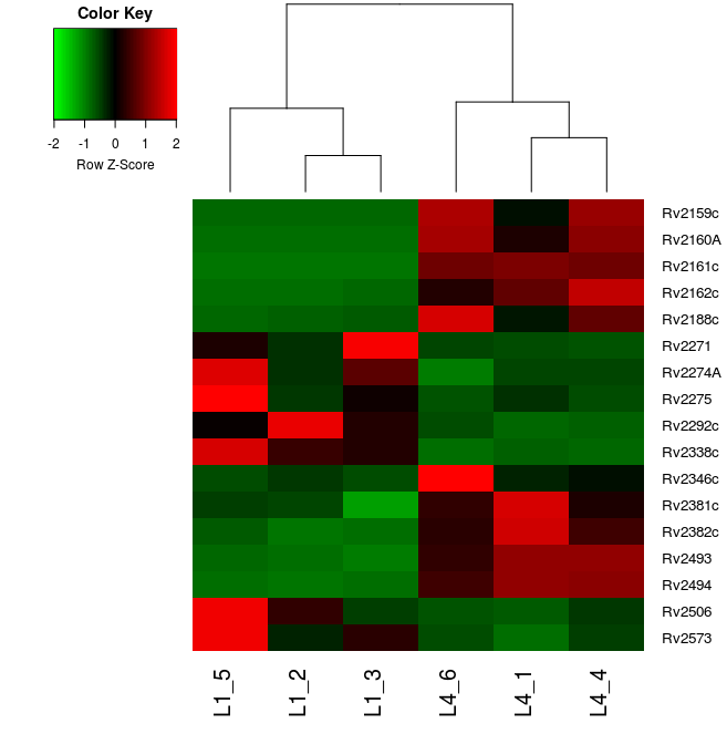
As you can see in the color key, red cells in the plot represent overexpressed genes whilst green ones the underexpressed genes. Rows represent the 17 genes of interest and columns the 6 samples we are analysing.

Further exploration

What do I do with a gene list?

As we have just seen, differential expression analysis results is a list of genes exhibiting different activities between two conditions. It can be daunting trying to determine what the results mean. On one hand you may find that due to there being no real differences or there being too much noise in your experiment, you have no significant differences. On the other hand, you may find thousands of differentially expressed genes. What can you say about that?

Other than looking for genes which you expect to be different or unchanged, one of the first things to do is look at Gene Ontology (GO) term or gene set enrichment. There are many different algorithms for this. For example, you could annotate your genes with functional terms from GO using Bast2GO (Conesa et al., 2005) and then use perhaps TopGO (Alexa et al., 2006) to determine whehter any particular sorts of genes occur more than expected in your differentially expressed genes. Another popular tool that has been tried and tested for a long time is GSEA

References

Mortazavi A, Williams BA, McCue K, Schaeffer L, Wold B. (2008). Mapping and quantifying mammalian transcriptomes by RNA-Seq. Nat Methods 5(7):621-8. doi: 10.1038/nmeth.1226

Wang Z, Gerstein M, Snyder M. (2009). RNA-Seq: a revolutionary tool for transcriptomics. Nat Rev Genet 10(1):57-63. doi: 10.1038/nrg2484

Cole ST, Brosch R, Parkhill J, Garnier T, Churcher C, Harris D et al. (1998). Deciphering the biology of Mycobacterium tuberculosis from the complete genome sequence. Nature 393(6685):537-44.

Parwati I, van Crevel R, van Soolingen D. (2010) Possible underlying mechanisms for successful emergence of the Mycobacterium tuberculosis Beijing genotype strains. Lancet Infect Dis 10(2):103-111. doi: 10.1016/S1473-3099(09)70330-5

Conesa A, Gotz S, Garcia-Gomez JM, Terol J, Talon M, Robles M. (2005) Blast2GO: a universal tool for annotation, visualization and analysis in functional genomics research. Bioinformatics 21(18):3674-6.

Alexa A, Rahnenfuhrer J, Lengauer T. (2006). Improved scoring of functional groups from gene expression data by decorrelating GO graph structure. Bioinformatics 22(13):1600-7.