GWAS - Pathogen 'Omics

GWAS lecture

Genome Wide Aassociation Studies (GWAS) Practical

The objective of this tutorial is to get you familiar with the basic file format used for GWAS and common tools used for analysis and take you through data Quality control (Crucial in any study!).

Our dataset is based on a GWAS study for Meningococcal disease in a European population (https://www.nature.com/articles/ng.640).

Data:

Genome wide SNP data
Scripts to facilitate analysis

Software you will need for analysis

Computer workstation with Unix/Linux operating system
PLINK software for genome-wide association analysis: http://pngu.mgh.harvard.edu/_purcell/plink/download.shtml
Statistical software for data analysis and graphing such as: R: http://cran.r-project.org/
SMARTPCA.pl software for running principal components analysis (not used in this tutorial to save time): http://genepath.med.harvard.edu/~reich/Software.htm
BCFtools

The software has been provided in a conda environment. Activate it with:

conda activate gwas

A. Create BED files for analysis:

1. Convert your plink genotype files to binary format - smaller file easier for manipulation of data

We have already provided you with plink formatted files we won't have to do this step.

plink allows for the conversion from many different formats to its own format. For example if you had a VCF file you could type:
plink --vcf MD.vcf.gz --make-bed --out MD

Your data set:

A plink-binary-formatted dataset consisting of 3004 individuals, 409 cases, 2595 controls, 601089 variants. The three files starting with MD. hold all the information plink needs:

MD.bed – binary-encoded information on individuals and variants
MD.bim – variant information: “Chromosome”, “Marker name”, “Genetic Distance” (or '0' as dummy variable), “Base-pair coordinate”, “Allele 1”, “Allele 2”. Each SNP must have only two alleles.
MD.fam – information on the individuals: The first 6 columns are mandatory and in the order: “Family ID”, “Individual ID”, “Paternal ID”, “Maternal ID”, “Sex”, “Phenotype”.

Double-check the basic stats of your dataset (number of variants, individuals, controls, cases) by examining MD.bim and MD.fam with bash utilities like awk or wc.

Click to expand hint

MD.fam holds one line per individual and MD.bim has one line per variant. We can therefore use the word-counting utility wc to get those numbers with

wc -l MD.{bim,fam}

Alternatively, you can count the number of lines with awk like so

awk 'END{print NR}' MD.bim
awk 'END{print NR}' MD.fam

In order to get the number of controls and cases ('1' and '2' in the 6th column in the .fam file, respectively), we can again use awk, which is very versatile:

awk 'BEGIN{contr=0;cases=0;FS=" "}
  {if($6==1){contr++} if($6==2){cases++}}
  END{print "control", contr; print "cases", cases}' MD.fam

However, awk's syntax can be quite intimidating to beginners. Instead, we can get the numbers of cases and controls by chaining together a few other programs like so:

cut -f 6 -d ' ' MD.fam | sort | uniq -c

This gets the 6th column of the MD.fam file and counts the occurrences of the unique values.

uniq expects sorted input. Try the command again without sort and see how the output changes.

B. Sample QC

1. Identification of Individuals with discordant sex information
Ideally, if X-chromosome data are available, we would calculate the mean homozygosity rate across X chromosome markers for each individual in the study and identify discordance with our reported sex phenotype.
As our data only contains autosomes we will skip this step.

2. Identification of individuals with elevated missing data rates or outlying heterozygosity rate

2.1. At the shell prompt type:

plink --bfile MD --missing --out MD

This creates the files MD.imiss (sample-based missing report) and MD.lmiss (variant-based missing report). The fourth column in the .imiss file (N_MISS) gives the number of missing SNPs and the sixth column (F_MISS) gives the proportion of missing SNPs per individual.

2.2. At the shell prompt type:

plink --bfile MD --het --out MD

This creates the file MD.het where the third column gives the observed number of homozygous genotypes [O(Hom)] and the fifth column gives the number of non-missing genotypes [N(NM)], per individual.

2.3. Calculate the observed heterozygosity rate per individual using the formula (N(NM) - O(Hom))/N(NM) and create a graph where the proportion of missing SNPs per individual is plotted on the x-axis and the observed heterozygosity rate per individual is plotted on the y-axis. We have provided an R script for this task. Run it by typing:

R CMD BATCH imiss-vs-het.Rscript

This creates the graph MD.imiss-vs-het.pdf (see below).

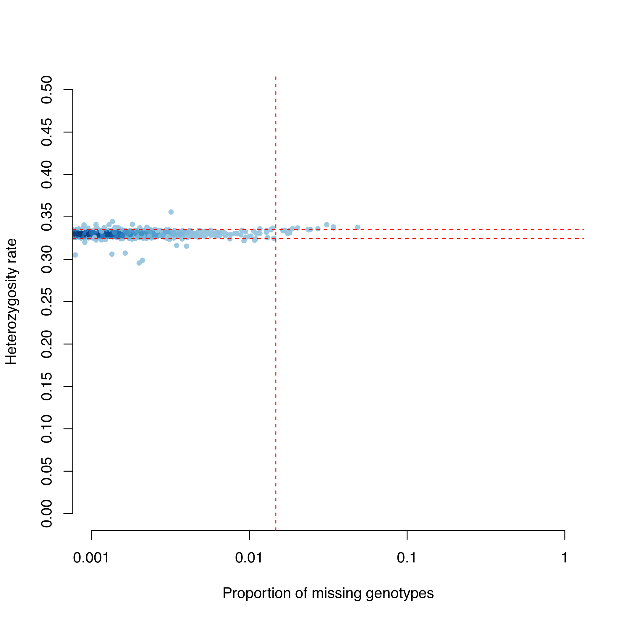
You can open the file by navigating your file browser in the correct directory and double clicking on it or by typing xdg-open MD.imiss-vs-het.pdf. This command will use the default program to open any file. If you would like to open the current directory in the file browser, you can type xdg-open ..

Examine the plot to decide reasonable thresholds at which to exclude individuals based on elevated missingness or extreme heterozygosity. Here we will exclude all individuals with a

genotype failure rate ≥ 0.0185 (vertical dashed line) and/or
a heterozygosity rate ± 3 standard deviations from the mean (horizontal dashed lines).

2.4. Extract the family ID and individual ID of all samples failing this QC using another R script:

R CMD BATCH imiss_het_fail.Rscript

This produces a file named fail_imiss_het_qc.txt.

How many samples failed this QC stage?

Click to expand answer

wc -l fail_imiss_het_qc.txt tells us that the file has 99 lines. Therefore, 99 samples failed this test.

3. Identification of duplicated or related individuals

3.1. To identify duplicates & related individuals, create an identity-by-state (IBS) matrix – calculated for each pair of individuals based on the shared proportion of alleles.

3.1.1. To reduce the computational complexity, first prune the dataset so that no pair of SNPs (within a given window e.g 200kb) has linkage disequilibrium (r² > 0.2). Type

plink --bfile MD --indep-pairwise 200 5 0.5 --out MD

This creates files with the extensions .prune.in, .prune.out, and .log.

3.1.2. Then, to extract the pruned SNPs and generate the pair-wise IBS matrix, type:

plink --bfile MD --extract MD.prune.in --genome --out MD

This might take a few minutes and then creates files with the extensions .genome & .log.

You can also create a BED file with the pruned SNPs: plink --bfile MD --extract MD.prune.in --make-bed --out MD.pruned

How many SNPs are in your pruned list?

Click to expand answer

You can have a look at your log file (using the less command) or type wc -l MD.prune.in, which should tell you that there are 260,787 SNPs in the pruned list.

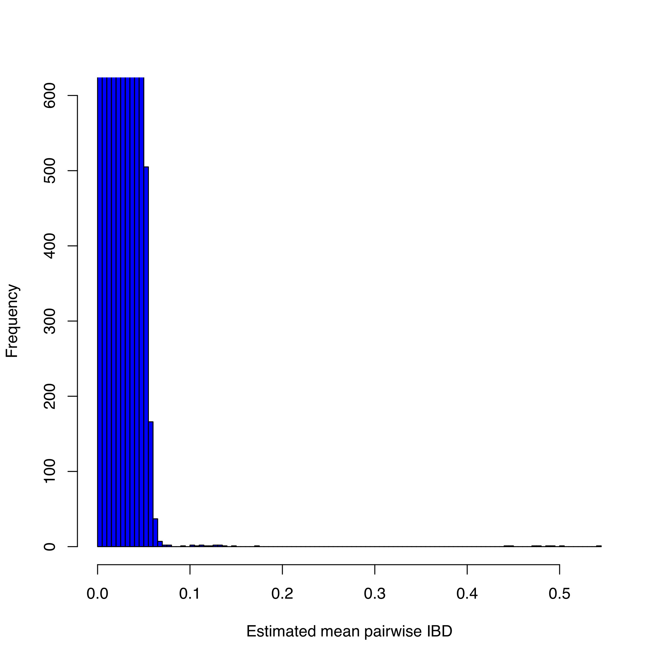
3.1.3. We have provided a Perl script in order to identify all pairs of individuals with an Idenity-by-descent (IBD) > 0.185. Invoke it with

perl run-IBD-QC.pl MD

The code also looks at the individual call rates stored in MD.imiss and outputs the ID of the individual with the lower call rate to fail_IBD-QC.txt for each pair of related individuals.

To visualise the IBD rates, type:

R CMD BATCH  plot-IBD.Rscript

this generates MD.IBD-hist.pdf:

Note: The expectation is that IBD = 1 for duplicates or monozygotic twins, IBD = 0.5 for 1st-degree relatives, IBD = 0.25 for 2nd-degree relatives and IBD = 0.125 for 3rd-degree relatives. Due to variation around these values it is typical to exclude one individual from each pair with an IBD > 0.185, which is halfway between the expected IBD for 3rd- and 2nd-degree relatives.

How many individuals fail to meet the IBD threshold? Hint: use the less command to view the file or wc -l filename to count the number of lines

Click to expand answer

8 samples failed the threshold.

4. Identification of individuals of divergent ancestry

In the interest of time, this step has been mostly done for you.

4.1. Principal components analysis (PCA) was performed with pruned bed file datasets generated from step 3.1.2 using the ./RUN_PCA.sh command. This generated the following output files (stored in PCA_files): MD.pruned.pca.par, MD.pruned.pca.log, MD.pruned.pca.evec, MD.pruned.pca, MD.pruned.eval. The file with the .evec extension file is what you will need to view your PCs.

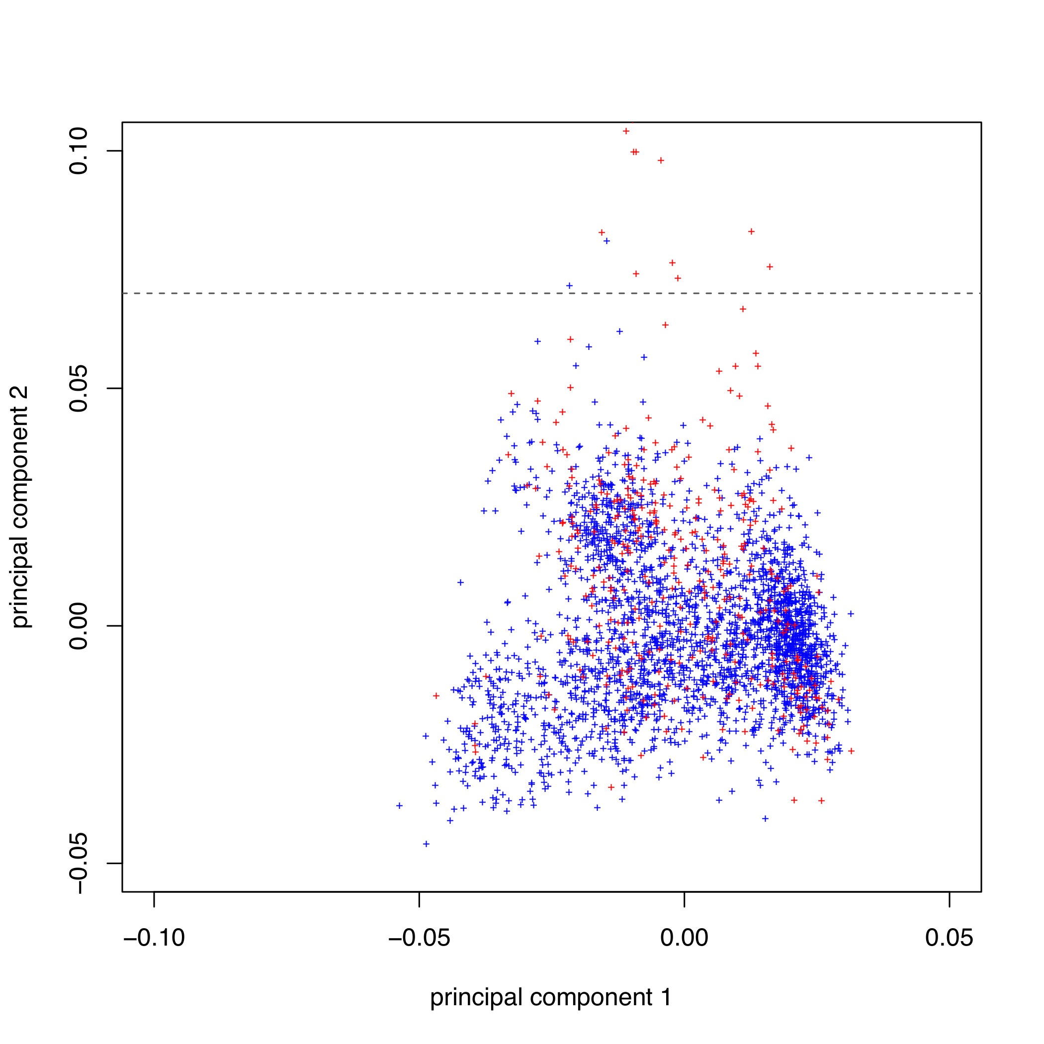
4.2. Create a scatter diagram of the first two principal components, including all individuals in PCA_files/MD.pruned.pca.evec (the first and second PCs are columns 2 and 3 respectively), using yet another R script. Type:

R CMD BATCH plot-pca-results.Rscript

This creates pca_plot.pdf:

Data in column 4 is used to colour the points according to phenotype (i.e. case vs control). Here, we chose to exclude all individuals with a 2nd principal component score >0.07.

Next we can run

R CMD BATCH write_pca_fail.R

to write the FID and IID of the filtered individuals to a file called fail_pca.txt.

How many individuals failed the PCA threshold?

Click to expand answer

wc -l fail_pca.txt tells us that 14 individuals were excluded in this step.

4.3. Remove all individuals failing QC

4.3.1. We can use the cat command to concatenate all the files listing individuals failing the previous QC steps into single file:

cat fail*txt | sort -k1 | uniq > fail_qc_inds.txt

The file fail_qc_inds.txt should now contain a list of unique individuals failing the previous QC steps.

4.3.2. To remove these from the dataset type:

plink --bfile MD --remove fail_qc_inds.txt --make-bed --out clean.MD

How many individuals in total will be excluded from further analysis?

How many individuals in total do you have for further analysis?

Click to expand answer

We could again use wc in order to count the number of lines in clean.MD.fam. Alternatively, you can use less clean.MD.log to have a look at the log-file of the previous step and extract the information from there. This should tell us that we have 2888 samples left which means that 116 were removed.

C. Marker QC

5. Identify all markers with an excessive missing data rate

5.1. To calculate the missing genotype rate for each marker type:

plink --bfile clean.MD --missing --out clean.MD

The results of this analysis can be found in clean.MD.lmiss.

5.2. Plot a histogram of the missing genotype rate to identify a threshold for extreme genotype failure rate. This can be done using the data in column five of the clean.MD.lmiss file. Use an R script provided for this task by typing:

R CMD BATCH lmiss-hist.Rscript

This generates clean.MD.lmiss.pdf

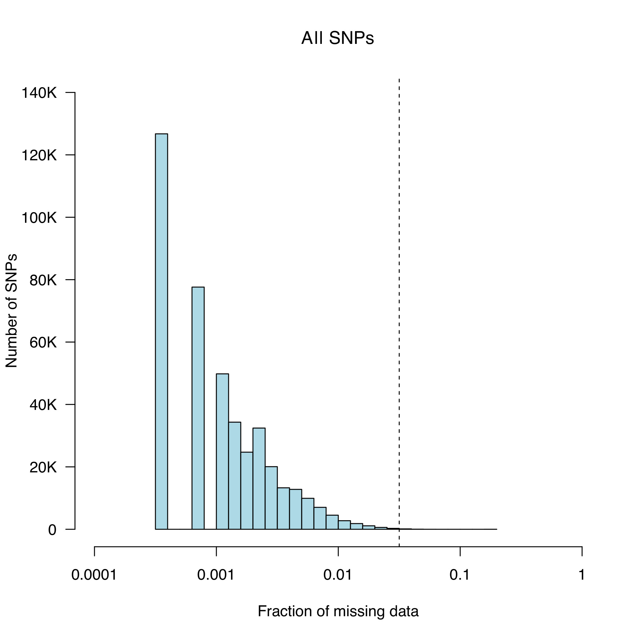
We chose to a call-rate threshold of 5% (these SNPs will be removed later in the protocol).

6. Test markers for different genotype call rates between cases and contols

6.1. To test all markers for differences in call rate between cases and controls, at the Unix prompt type:

plink --bfile clean.MD --test-missing --allow-no-sex --out clean.MD

The output of this test can be found in clean.MD.missing.

To create a file called fail-diffmiss-qc.txt, which contains all SNPs with a significantly different (P<0.00001) missing rate between cases and controls, type

perl run-diffmiss-qc.pl clean.MD

How many variants have failed QC?

Click to expand answer

wc -l fail-diffmiss-qc.txt shows us that 400 variants were selected to be removed.

7. Remove all markers failing QC

7.1. To remove poor SNPs from further analysis and create a new clean (QC'D) MD data file, at the Unix prompt type:

plink --bfile clean.MD --exclude fail-diffmiss-qc.txt --maf 0.01 --geno 0.05 --hwe 0.00001 --make-bed --out clean.final.MD

In addition to markers failing previous QC steps, those with a MAF < 0.01, missing rate > 0.05 and a HWE P-value < 0.00001 (in controls) are also removed.

How many variants and individuals pass filters and QC for your GWAS?

Click to expand answer

Have a look at clean.final.MD.log. Towards the end of the file you will find the following line:

597518 variants and 2888 people pass filters and QC.

8. Perform a GWAS on your QC'ed dataset

8.1. To run a basic case/control association test, at the unix prompt type:

plink --bfile clean.final.MD --assoc --ci 0.95 --adjust --allow-no-sex --out final.MD.assoc

Your association output file will contain 12 columns:

CHR Chromosome SNP SNP ID BP Physical position (base-pair) A1 Minor allele name (based on whole sample) F_A Frequency of this allele in cases F_U Frequency of this allele in controls A2 Major allele name CHISQ Basic allelic test chi-square (1df) P Asymptotic p-value for this test OR Estimated odds ratio (for A1, i.e. A2 is reference) L95 Lower bound of 95% confidence interval for odds ratio U95 Upper bound of 95% confidence interval for odds ratio

8.2. To visualise your data:

We will use another R script to generate two more plots:

8.2.1. A Quantile-Quantile (QQ) plot of your p-values to look at the distribution of P-values and assess whether genomic inflation is present (lambda>1) (this can also be found in your .assoc.log file).

8.2.2. A Manhattan plot to visualise where your association signals lie across the chromosomes. Type:

R CMD BATCH GWAS_plots.R

This generates both plots: final.MD.assoc_qq.png and final.MD.assoc_mhplot.png

What do the plots tell you?

Click to expand answer

There appears to be some genomic inflation (as was also indicated by the estimated inflation factor of 1.08 in the log-file). However, overall the p-values are well behaved, but there are no variants that make it past the significance threshold of 5×10^-8. This might be due limited power given our relatively small sample size (approx. 3000 individuals with 500 cases). Some towers, however, come relatively close. One of those will be discussed in more detail below.

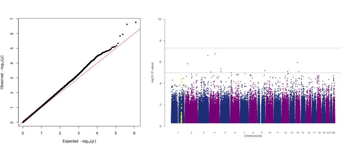
8.2.2.1. Let's zoom into a region of interest: the tower of SNPs on CHR1 (coloured in yellow). This the Complement Factor H (CFH) region known to be associated with Meningococcal disease. The previous Rscript in 8.2.2 above also generated the chr1_CFH_region.txt file.

Open the locuszoom webpage: http://locuszoom.org/genform.php?type=yourdata
Upload the text file and select PLINK data format.
Enter the most associated snp (“rs1065489”) with a flanking size of 500KB
In the Genome Build/LD Population field select the appropriate hg19 european ref panel.
Then press "Plot Data" to generate your plot.